
When you need to find information in a large spreadsheet or you’re always looking for the same kind of information, you can save time using the VLOOKUP function in Excel.
VLOOKUP works a lot like a phonebook, where you start with some information you know (such as someone’s name) and use it to find some data you don’t know (such as their phone number).
How to use VLOOKUP
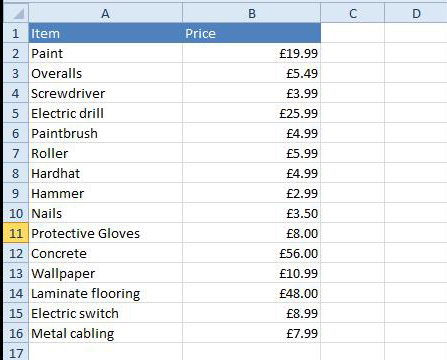
Here is an example of how you might use VLOOKUP to find the price of one particular product in your product list – Laminate flooring. You can probably already see from the screen shot below that the price is £48.00, but that’s because this spreadsheet is a simple example. Once you learn how to use VLOOKUP, you’ll be able to use it with larger, more complex spreadsheets, and that’s when it will become truly useful.
Getting the formula started
We’ll add our formula to cell E2, but you can add it to any blank cell. As with any formula, you’ll start with an equals sign (=). Then type the formula name. Our arguments will need to be in brackets, so type an open brackets. So far, it should look like this:
=VLOOKUP(
Adding the arguments
Now, we need to add 4 arguments that will tell VLOOKUP what to search for and where to search.
The first argument is the name of the item you’re searching for, which in this case is Laminate flooring. Because the argument is text, we’ll need to put it in double quotes:
=VLOOKUP(“Laminate flooring”
The second argument is the cell range that contains the data. In this example, our data is in A2:B16. As with any function, you’ll need to use a comma to separate each argument:
=VLOOKUP(“Laminate flooring”, A2:B16
Note: It’s important to know that VLOOKUP will always search the first column in this range. In this example, it will search column A for “Laminate flooring”. In some cases, you may need to move the columns around so the first column contains the correct data.
The third argument is the column index number, which is simpler than it sounds: The first column in the range is 1, the second column is 2, etc. In this case, we are trying to find the price of the item, and the prices are contained in the second column. This means our third argument will be 2:
=VLOOKUP(“Laminate flooring”, A2:B16, 2
The fourth and final argument tells VLOOKUP whether to look for approximate matches, and it can be either TRUE or FALSE. If it is TRUE, it will look for approximate matches. Generally, this is only useful if the first column has numerical values that have been sorted. Because we’re only looking for exact matches, the fourth argument should be FALSE. This is our last argument, so go ahead and close the parentheses:
Your finished formula should now read:
=VLOOKUP(“Laminate flooring”, A2:B16, 2, FALSE)
That’s it! When you press Enter, it should give you the answer, which is £48.00.