
Drilling down to the figures you most need can be tricky when you are working with a bulky Excel spreadsheet. But by filtering large quantities of data, you can choose to display only the rows that meet specific criteria or simply hide the rows you do not want to see.
Once your filter is applied, you can then easily copy, edit, format and print the subset of filtered data without rearranging or moving it.
Here are a few of the ways to filter your data in Excel:
Filter data in a table
When you put your data in a table, filtering controls are added to the table headers automatically.
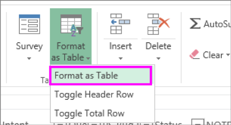
- Select the data you want to filter. On the Home tab, click Format as Table, and then pick Format as Table.
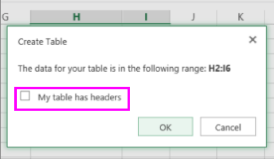
2. In the Create Table dialog box, you can choose whether your table has headers.
- Select My table has headers to turn the top row of your data into table headers. The data in this row won’t be filtered.
- Don’t select the check box if you want Excel Online to add placeholder headers (that you can rename) above your table data.
- Click OK.
- To apply a filter, click the arrow in the column header, and pick a filter option.
Filter a range of data
If you don’t want to format your data as a table, you can also apply filters to a range of data.
- Select the data you want to filter. For best results, the columns should have headings.
- On the Data tab, choose Filter.
Filtering options for tables or ranges
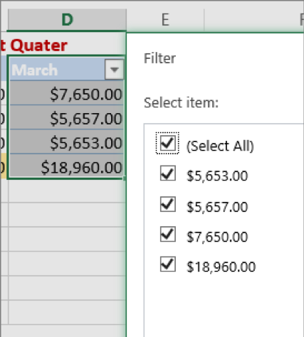
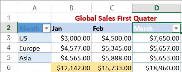
You can either apply a general Filter option or a custom filter specific to the data type. For example, when filtering numbers, you’ll see Number Filters, for dates you’ll see Date Filters, and for text you’ll see Text Filters. The general filter option lets you select the data you want to see from a list of existing data like this:
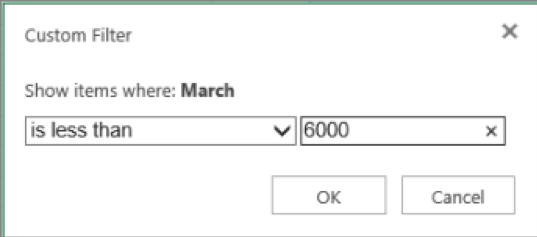
Number Filters lets you apply a custom filter:
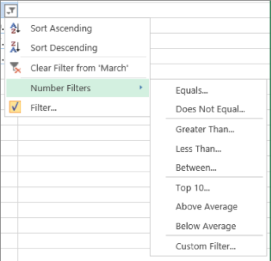
In this example, if you want to see the regions that had sales below $6,000 in March, you can apply a custom filter:
Here’s how:
- Click the filter arrow next to March > Number Filters > Less Than and enter 6000.
- Click OK.
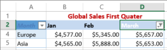
Excel Online applies the filter and shows only the regions with sales below $6000.
You can apply custom Date Filters and Text Filters in a similar manner.